Violin backs are typically made of maple that has distinctive horizontal stripes called flame. The flame, also known as curl or figure, is caused by the reflection of light at different angles that creates a pleasing visual effect of rolling waves. Violin makers can orient the flame in different configurations depending on the constraints of the tonewood and according to their preferences: Some prefer backs made in a single piece of wood; others prefer two-piece backs with flame either ascending or descending from the center joint to the edges. In the first of a two part Carteggio, computer scientist Pierre Adda describes how he built software to classify the flame orientation of violin backs in Tarisio’s extensive photo archive. Next week, in part two, Jason Price examines this data and draws generalizations and conclusions about makers’ tendencies and preferences regarding wood choice.
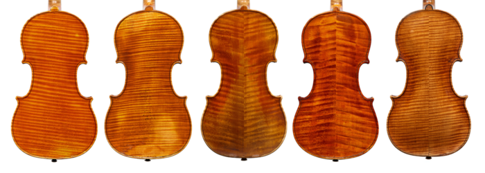
Figure 1: Illustration of the variety of violin’s back appearances.
Writing software to detect and determine the angle of the flame on the back of a violin, even in an approximate manner, is a challenging task. No two flames are the same; they vary in form, size and intensity, which can pose difficulties in accurately identifying and outlining them. Plus, a three-hundred-year-old violin’s back isn’t always pristine, and scratches or other textures can further complicate the detection process. Therefore, developing an effective and robust way to consistently detect wood flames is crucial.
We decided to use a classic computer vision approach. Line detection has long been used in computer vision; we specifically selected the Hough line detection algorithm, which we then modified into a weighted Hough algorithm to better suit the wood flame detection task.
In addition, we utilized two deep learning models which we developed previously for Tarisio applications, specifically the c-bout keypoint detection model and the one-piece / two-piece back classification model, to assist us in this task. These models help identify the region of interest on the back of the violin.
Because these concepts can be confusing, I’m going to start by explaining how Hough line detection works, followed by a short explanation of image preprocessing, which plays a crucial role in identifying wood flames. That way, when it comes to explaining the modified Hough algorithm and its implementation, the results—and their significance—will be clear.
Hough Line Detection
The Hough Transform is a popular classical computer vision algorithm that can be used to detect various shapes, but is primarily used to detect prominent lines in an image even if they are broken or incomplete. The technique we used to detect wood flames is a modified version of the “Hough line detection” algorithm.
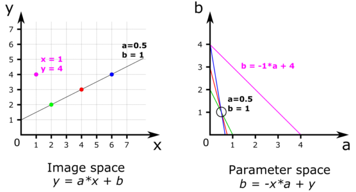
Figure 2: Basic principle of Hough transformation and line detection with only 4 pixels. The coordinates of the pixels in the image space are used to draw lines in the parameter space. Intersecting lines in the parameter space indicate that a line in the image space passes through multiple pixels.
The first step in line detection is to transform the image in order to outline the edges and obtain a skeletonized image (see Figure 3-e). This process will be further explained in the next chapter on image preprocessing. In a skeletonized image, all pixel values are set to 0, except for the edge pixels (e.g. the outline of an object) which are set to 1. The objective of line detection is to identify straight lines that pass through a maximum number of edge pixels, and the Hough transform allows us to do just that.
If we were able to register in a table all possible lines going through each edge pixel, it would then be possible to identify recurring lines and count their occurrence. It would then be easy to pick up the lines that appear most frequently.
This can sound impossibly tedious, but this is precisely what the Hough transform allows us to do, using a clever trick. This trick, illustrated in Figure 2, involves transforming the edge pixels from the image space into lines in the Hough parameter space. Let us elaborate on that:
In high school we learn that lines are defined by their equation y = a*x + b, where {x, y} are the coordinates and [a, b] represent the line’s “slope” and “intercept”. A pixel is defined by its coordinates {x, y} while a line is defined by its parameters [a, b]. The equation of a line can be transformed into b = -x*a + y , which is the same equation but presented as if [-x, y] were the parameters of a line and {a, b} were the coordinates of a point in a new space called the parameter space. Since we know the value of x and y in the image space, we can draw a line with a slope x and an intercept y in the parameter space. This is the clever trick! This line consists of an infinity of pixels with coordinates {a, b}, and each of these pixel coordinates represents the parameters of a line in the image space, a line that passes through the pixel {x, y}. We can repeat this operation for each edge pixel, resulting in several lines in the parameter space, as shown in Figure 2-b. When lines cross in the parameter space, it indicates that a single line [a, b] passes through multiple pixels {x, y}. In Figure 2-b, we can see that the three lines corresponding to the blue, red and green pixels cross at a single point a = 0.5 and b = 1, these values corresponding conveniently to the line that goes through all three pixels.
In practice, a computer program uses the edge pixel coordinates to draw lines on what is called an “accumulator”. Each line in the accumulator is given a value of 1, and when lines cross, the values add up at the intersection. These incrementing pixel values are usually named “votes”. In Figure 2-b for example, every line has a value of 1 except at the intersection of the blue, red and green lines where the value is 3 and at the intersection of the blue and purple lines where the value is 2. The highest value of the accumulator corresponds to the pixel with coordinates a=0.5 and b=1, which has 3 votes.
With an image containing hundreds of edge pixels, the accumulator would have hundreds of lines crossing one another. In this case, we would select the highest values in the accumulator using a given threshold, such as half of the maximum value. The coordinates of these values correspond to the prominent lines in the image. An accumulator can be seen in Figure 7, where the cartesian coordinates [a, b] have been replaced by polar coordinates [rho, theta].
Image Preprocessing
Carefully designed image preprocessing is crucial in order to apply the Hough line detection algorithm. Indeed, an image needs to be transformed into a binary skeletonized image. In a binary image, pixel values are either 0 or 1, with 0 representing the background and 1 representing the pixels of interest, i.e. the dots you see in Figure 2. For our specific case, an ideal binary skeletonized image of a violin’s back would contain the background set to 0, and the flames themselves represented by a 1-pixel line. This preprocessing pipeline is illustrated in Figure 3. The violin in Figure 3 is considered “easy”, with a lot of well defined flames.
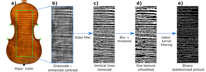
Figure 3: Image preprocessing pipeline for Hough line detection. The green circles represent the c-bout keypoints, which are used to define the region of interest.
To detect the flames, we must first define a region of interest on the violin’s back. This is done by utilizing the c-bout key points—that is, the coordinates that create the green rectangle in figure 2-a—that were previously predicted by our keypoint detection model.
Once this rectangular region of interest has been isolated, the image can be converted to grayscale and its contrast enhanced using the CLAHE algorithm (see Figure 2-b). This process not only highlights the flames but also standardises the images.
Next, we applied an edge detection filter, in this case, the Sobel filter, which effectively highlights areas where pixel values change rapidly. The filter can also remove vertical lines, which are often overlaid on wood flames, as shown above in Figure 3-c.
The output of the Sobel filter can be grainy but still contains important details. This “noisy” output can interfere with the functioning of the Hough line detection algorithm by introducing unwanted pixels in the skeletonized image. To address this, an additional preprocessing step is taken, which is what you see in Figure 3-d.
Finally, we applied a Gabor filter with specific values. The flames, which had been outlined in the previous preprocessing steps, now appear as one-pixel lines. This enables the image to be processed by the Hough line detection algorithm.
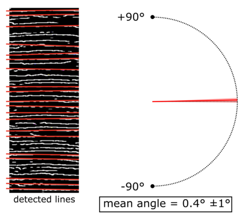
Figure 4: Lines detected by the Hough line algorithm (highlighted in red) on the skeletonized image from figure 3. The mean angle of these lines is 0.4°, with 0° representing a horizontal line. The standard deviation of the angles is 1°
Based on our previous deep learning model, we can now determine whether the violin is in one or two pieces. If it is in two pieces, we can easily run the Hough line algorithm on the left and right pieces separately.
The Hough line algorithm identifies the straight lines with the highest number of votes (see Figure 4). To eliminate lines that are too similar, a non-maximum suppression (NMS) algorithm is applied and a score threshold is used so as to retain only the lines that have more than half the votes of the line with the maximum number of votes. The resulting lines provide us with an average angle, a median angle and an angle standard deviation.
On a violin that is considered “easy” such as the one shown in Figures 3 and 4, the standard deviation of the angles generally ranges from 1° to 5°. However, on a more challenging violin, this standard deviation can be much larger. Empirically, we have found that the angle standard deviation can be interpreted as an error probability. A larger standard deviation indicates a higher likelihood of an incorrect result.
Based on the standard deviation numbers, we estimate that this preprocessing, along with the standard Hough line algorithm, yields approximately 80% correct results on the entire dataset. To hone these results we developed a modified version of the Hough line algorithm.
Weighted Hough Line Detection
Before delving into the workings of the weighted Hough line, let’s take a look at an example where preprocessing plus the standard Hough line algorithm don’t perform well. Figure 5 illustrates such a violin.
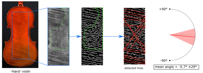
Figure 5: Line detection on a challenging violin. Highlighted in green is a patch of wood where the flames are not visible. The preprocessing filters captured random texture and scratches, leading to numerous unwanted detected lines and a significantly large angle standard deviation.
Although this violin back does have some visible flames, on a large patch of the cropped image, no flames are visible, as shown in the green area in Figure 5. Due to the nature of the filters used in preprocessing, random scratches and texture are captured resulting in the many little lines in the skeletonized image, while the flames are correctly captured as long continuous lines. Although the Hough algorithm successfully detects the flames, the presence of the small lines reveals the detection of numerous incorrect lines. Consequently, this leads to a significantly large standard deviation (in this case 29°). In most cases, a standard deviation exceeding 15° indicates an incorrect mean angle prediction.
To address this, we decided to assign weights to pixels in the skeletonized image based on the length of the line to which they belong. For instance, if a line consists of 10 connected pixels, we assign a value of 10 to every pixel of that line. The square root is here to reduce the difference between long and short lines, and we give weights to the pixels by utilizing a connected component algorithm. Doing so allowed us to obtain a skeletonized image with weighted pixels like that in Figure 6-a.
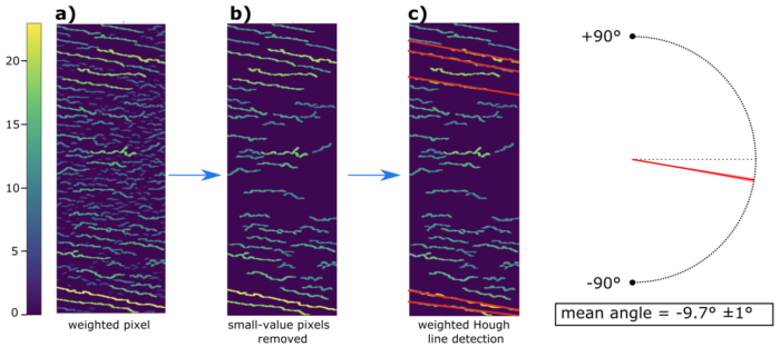
Figure 6: a) The skeletonized image from figure 5 with pixels weighted based on the length of the line to which they belong; b) pixel with small values are removed; c) modified weighted Hough line detection is applied, only the prominent lines are detected. This whole process results in a much more accurate angle prediction, with a standard deviation of only 1°.
With an image like this, it is easy to retain only the most prominent lines. This is done by calculating the median value of all non-zero pixels, and then setting all pixels below this value to zero. This step effectively eliminates a significant amount of unwanted noise, as demonstrated in Figure 6-b.
This technique alone can greatly enhance results, but we took it a step further by introducing the weighted Hough line algorithm. The concept is simple: In the standard Hough line algorithm, a line receives one vote for each pixel it passes through. In the weighted Hough line algorithm, the vote is weighted by the value of the pixel. As a result, only the prominent lines are detected, as shown in Figure 6-c. This leads to much more precise results. For the particular violin used in Figures 5 and 6, the standard deviation went from 29° to 1°, as only actual flames were detected.
Sliding Window Hough Line
Even after applying the technique described earlier to filter out the smallest lines, there may still be other issues when there is a high density of somewhat horizontal flames, as in Figure 3. In some cases, we observed that lines are incorrectly detected across multiple flames as they pass through numerous high-value pixels belonging to different flames. These incorrect lines typically have a relatively steep angle since they pass through several flames.
Limiting the angular scope of the Hough light detection is one way to address this problem. We can, for instance, restrict the detection to lines that deviate from the horizontal by less than 20°, but this prevents the detection of flames with steep angles. Although violins with steep-angled flames are rare, we want our algorithm to detect them since this is useful when identifying unusual violins.
Instead, we’ve proposed an alternative approach to Hough line detection. Rather than restricting the angular range, we have limited the spatial range by utilizing a sliding window technique; this is depicted in Figure 7. The Hough line algorithm is applied to a subsection of the image, which has the same width but a smaller height compared to the original image. In Figure 7, the subsection corresponds to one-third of the image height. The accumulator for this subsection is computed, and then the window slides down the image with a stride equal to half of the window’s height. The accumulator for this new window is added to the previous accumulator. This process is repeated until the window reaches the bottom of the image. The final accumulator is the sum of all accumulators and can be further processed.
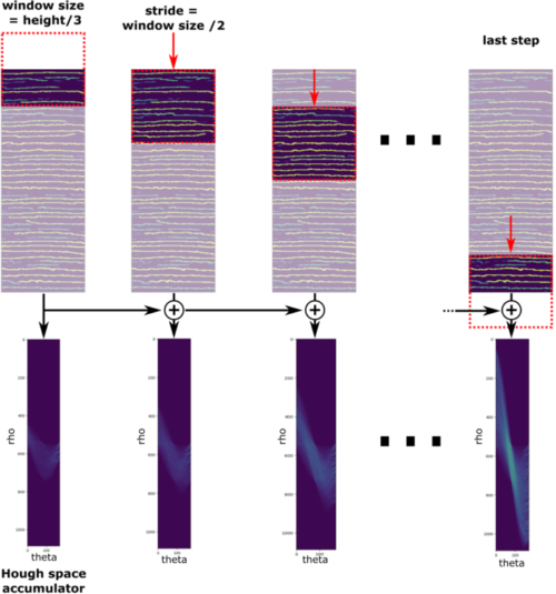
Figure 7: Hough line detection using a sliding window with a height equal to one-third of the image’s height. The Hough space accumulator of each window is summed to obtain an accumulator for the entire image.
Results
As previously mentioned, we found that the standard deviation of the detected angle serves as a reliable indicator of the accuracy of the angle prediction. To quantify this relationship, we manually reviewed the results for different standard deviation ranges. For each range, we randomly selected 200 images and determined the ratio of good predictions to bad predictions. This ratio was then considered as the error probability for that particular standard deviation range. From these results, we deduced a conversion law that relates the standard deviation to the error probability (see Figure 8-a).
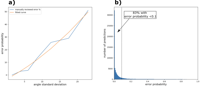
Figure 8: a) Correlation between the standard deviation of the detected angles and the error probability. b) Distribution of error probabilities across the dataset.
By converting the standard deviation into error probability for the entire dataset, we can generate a visualization of the error probability distribution (Figure 8-b). From this distribution, we observe that over 83% of all predictions have an error probability of less than 10%, and around 91% have an error probability of less than 20%. Overall, we can estimate that approximately 94% of all predictions are correct. It is worth noting that around 75% of predictions with an error probability exceeding 60% are from violins that do not have visible flames, at least not within the cropped rectangle where the hough line detection is applied (see Figure 3). Figure 9 showcases some examples of such violins.
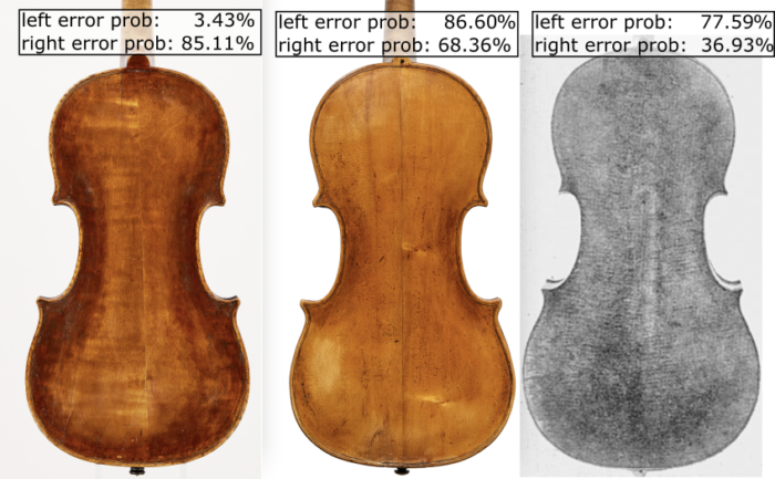
Figure 9: Three examples of violins where the algorithm failed to detect lines. On the first violin, the algorithm correctly detected flames on the left side, but failed to detect any flames on the right side. The second violin does not have any visible flames. The third violin, which has low resolution, exhibits very faint and dense flames that were not detected by the algorithm.
Conclusion and Prospects
Although the presented weighted Hough line detection algorithm is remarkably robust and effective with ~94% correct predictions, it does have certain limitations. The parameters used for image preprocessing aim to outline the flames and eliminate any other elements. As such, these parameters are a compromise between pixel gradient sensitivity and texture filtering. Accordingly, in certain cases, such as the third violin in Figure 8, the flames are not accurately distinguished from the surrounding elements. Additionally, due to the absence of direct confidence scores for line detection, there is no reliable approach to distinguish a violin without visible flames from a violin where the algorithm failed for other reasons. There are also rare instances of violins with diverging flames, where the orientation of the flames at the top of differs significantly from those at the bottom. In such cases, the algorithm will accurately detect the lines but will yield a high standard deviation/error probability for the angle.
One potential solution to address these challenges would be to utilize the predictions of the Hough line detection algorithm with a minimal error probability to train a deep learning model. This model could be designed by incorporating a feature-extracting backbone, followed by a multi-layer perceptron, and concluding with a classification layer with a sigmoid activation function. The classification can be based on bins representing different angle ranges, spanning from -90° to +90°, although the resolution of these bins is yet to be determined. However, there remains ongoing questions regarding this approach: If a model is trained on simpler examples (those with a low error probability), can it accurately predict outcomes for more challenging examples? Moreover, should we employ the raw output of the Hough line detection to train the model (multiple lines/angles), or solely rely on the mean or median angle? Nevertheless, this approach holds promise as a means to further enhance the results.
Pierre Adda is a computer scientist specializing in computer vision. He holds a master’s degree in physics and a PhD in electrical engineering. Aside from his work with computers, Pierre is also a musician with over 20 years of training in classical piano. He has also played guitar in several bands in Paris.
Next week, in part two, Jason Price examines the data that Pierre generated and draws generalizations and conclusions about makers’ tendencies and preferences regarding wood choice.